Yeah, I'm Thinkin I'm Back
Tim Goes Back to College
This was a working month. My classes started to pick up and I more seriously examined corpus management strategies and digital text analysis techniques. My reading was thus quite technical in nature. I’ll be brief.
-
Mahesh Joshi, Dipanjan Das, Kevin Gimpel, Noah A. Smith, Movie Reviews and Revenues: An Experiment in Text Regression
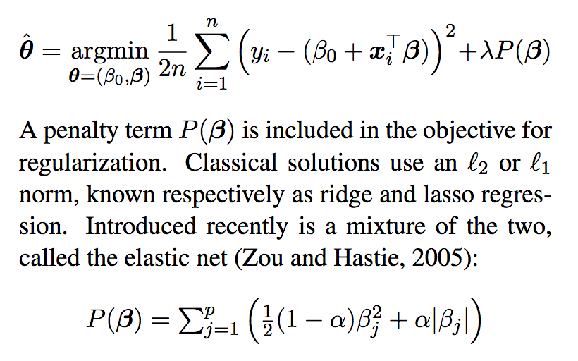
The authors set out to predict a Hollywood movies opening weekend revenue. This connects well with the work carried out by Archer and Jockers since they look for commonalities in the most popular instances of their medium. The regression technique is what drew me to the paper. It was introduced to me in my Machine Learning class with Professor Qi. Indeed, to analyze the wealth of metadata they collect (stored in .XML files), they carry out a regression known as “elastic net.” Elastic Net is a mixture of ridge and lasso regularization.

Regularization is the process of shrinking the parameters of your predictive model in order to balance irregularities inherent in your data set. Ridge regression is helpful because it is easy to implement. You introduce the L2 Vector norm into your regression equation. I even implemented it for homework this week in Python.
#Beta Star = (X_t dot X + Lambda * Identity) inv.. dot (X_t dot y)
xMat_t = np.transpose(xVal)
xResultMat = np.matmul(xMat_t, xVal)
lMat = lambdaV * np.identity(3)
plus = np.add(xResultMat, lMat)
invQuant = np.linalg.inv(plus)
xMat_tDotY = np.matmul(xMat_t, yVal)
beta = np.matmul(invQuant, xMat_tDotY)
Lasso Regularization is another “shrinking” method when carrying out regression but introduces a non-linear parameter, the L1 Vector norm, into your work. This is an efficient way to carry out feature selection in order to determine what columns in your data matrix are significant. The brilliance of Elastic Net is you take advantage of the benefits of both regularization techniques. The
glmnetpackage in R provides simple steps for implementation of Elastic Net.The results of this study conclude that a subset of words in movie reviews possess a heightened significance when it comes to the box office potential of a movie. For instance, the authors conclude that “documentary” penalizes a movie’s potential by .037 U.S. Dollars per occurence, while “Will Smith” raises your movie’s potential by more than $2.560 a mention. A reason, then, to “Hitch” your bets on any movie containing Mr. Smith.
This paper provides a salient framework for feature analysis of a traditionally overlooked corpus in order to solve a compelling and challenging problem. I will potentially draw upon it in my work. I am still not sure if I am going to use regression analysis or a different learning algorithm like KNN or SVM. More to come on that, for sure.
-
Jodie Archer and Matthew Jockers, The Bestseller Code: Anatomy of the Blockbuster Novel
Archer and Jockers set out to define what makes a New York Times Bestseller tick. This places the work in direct relation to the aim of this thesis. I will leave aside some of their easier to pull out conclusions in order to briefly discuss the work’s technical aspects. (I plan to include a more thorough overview of the work in my thesis proper).
After alaborious text cleaning process, Jockers and Archer are left with 28,000 features. By features I mean a conrete data point that could be relayed to you using a matrix or vector. Staggering on its face, the 28,000 number is by no means a standard of proof or burden for my project. Indeed, I would be happy if I could accurately tease out 50 or so numerical data points about my corpus. They ultimately reduce their list to 2799 features in methods only vaguely explained as using “machine learning and classification experiments” … which could mean anything. Frustrating as this is I still continue on in their explanation to help craft the types of techniques I can use for my work.
To take advantage of their pared down their massive feature list, they rely on KNN (K-Nearest Neighbors).
KNN is perhaps the simplest type of “Machine Learning” one can carry out because you never actually construct a model when using it. Instead, you plot your training set of data onto a plane. Next, I would plot one of my testing points – one of my unknowns – onto the graph. In order to determine what class it falls into I would inspect the most-common class of the points inside its “neigborhood,” the k points it is closest to (using a measure like Euclidean distance).
So, across a space of 2799 dimensions they use KNN to determine a simple enough binary: whether or not a work is a bestseller or not. And they were correct 90% of the time. Not too bad for a couple thousand lines of R Code!
I will continue working with my professors and lots of Google/JSTOR searches to look for the best ways to carry out feature analysis. This work as whole, though, provides a compelling explanation of the similarities and differences across a large class of works that share an amorphous label. It will be of immense value for my work.
Looking forward I hope to start adding some “reading” of my model outputs onto posts such as these. I would love, for instance, to have my Halloweekend be interrupted by a spooky and lugubrious mess of Data Frames I need to parse through. Here’s to hoping October provides growth and development for the project!